Comparison Between Xfoil & RANS CFD Aerodynamic Predictions - 2D Airfoil

           Overview and Objectives

This project aimed to compare the relative accuracy of several different RANS models compared to the viscous/inviscid methods of Xfoil, which was indirectly derived from the XFLR5 program. Several different airfoils with varying levels of thickness, camber, and leading edge radii were chosen so as to better represent the diversity of airfoils out there. It is important to note that this analysis is only focused on the incompressible & subsonic regimes, which tends to favor viscous/inviscid methods due to their alleged increased robustness in predicting transition and such, at least this is what the author currently understands the situation to be. The results will be compared to experimental data cited in the book “Theory of Wing Sections” by Albert E. Von Doenhoff and Ira Abbott. The author used the “web plot digitizer” program to get actual values from the graphs in the aforementioned book to the best of his abilities.

• Reynolds Number: 9,000,000
• k-⍵-SST, k-e Realizable & Spallart Almaras RANS turbulence models
• XFLR5 (Xfoil) employment
• Steady state solution: final time step
• Static pressure: P∞=101325 Pa = 1 atm
• Static temperature: T = 300 K
• Incompressible: Mach = 0.01
• Airfoil dimensions: L = 1 m (chord length), NACA 0006 & 2421
  

               Mesh Details

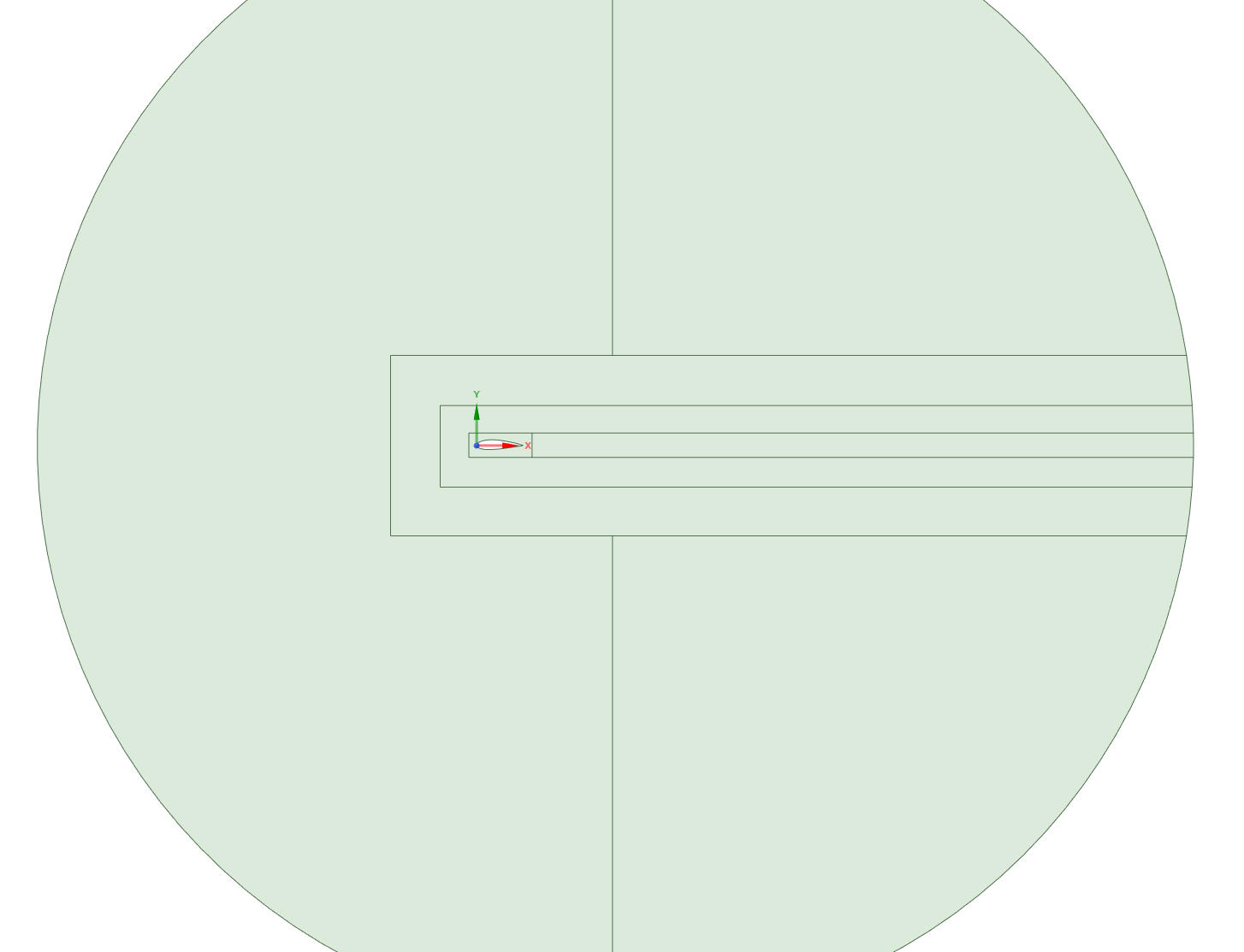
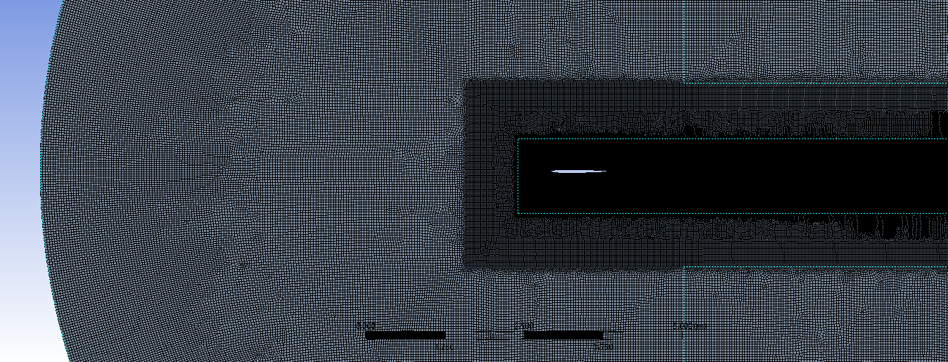
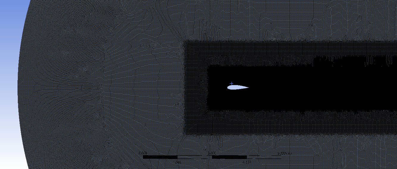
The mesh will be defined with 4 blocks; 1 block at the very inside of the domain, closest to the airfoil, 1 block at the very outside of the domain, farthest from the airfoil at the boundary, and 2 additional blocks to break up the center between the other 2. In regards to spatial convergence, an ultra high resolution, which given the author’s experience is more than enough for convergence of lift and drag values, was employed instead of using several different mesh resolutions. This was done because making structured meshes in 2D actually takes nearly as much time as actually solving the numerical problem. As such, it would actually take less time to make one overkill mesh and solve that than to perform traditional mesh convergence. Figure 1 showcases the domain and block geometry. The left side is the inlet and the right side is the outlet. The inner four inner, long rectangular regions around the airfoil are the blocks and the remaining space is called “Rest of Domain.”

           Table 1: Mesh Block Information

       Table 2: Number of Cells for each Airfoil Case

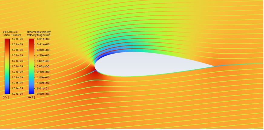
        Visualization: Pressure & Velocity Contours

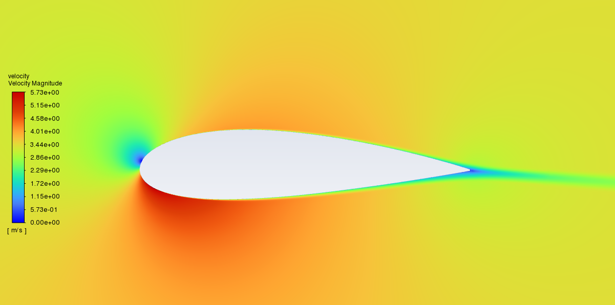
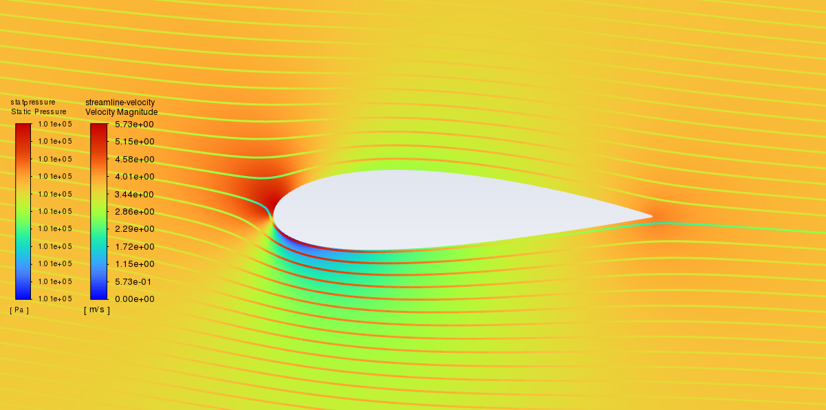
Figure 4&5: Velocity (L) & Pressure (R) Contours - NACA 2421 - AoA -6

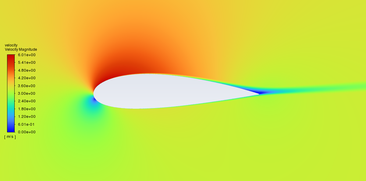
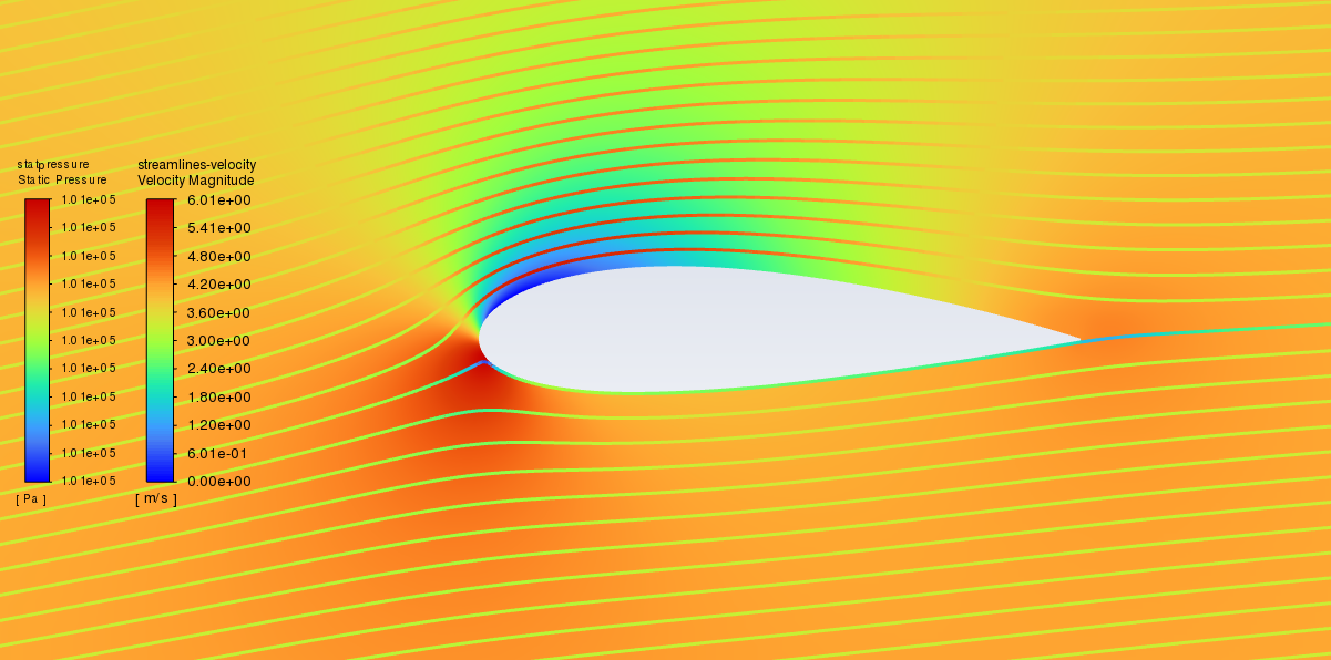
Figure 6&7: Velocity (L) & Pressure (R) Contours - NACA 2421 - AoA 8

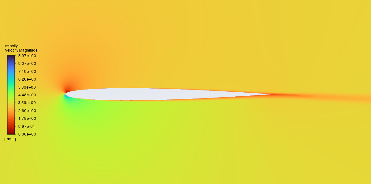
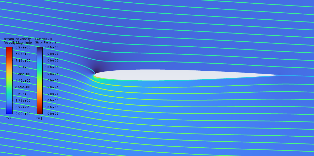
Figure 8&9: Velocity (L) & Pressure (R) Contours - NACA 0006 - AoA -6

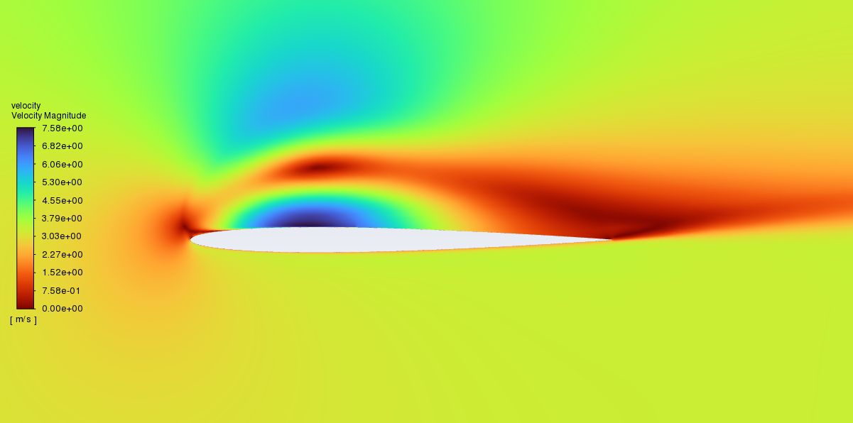
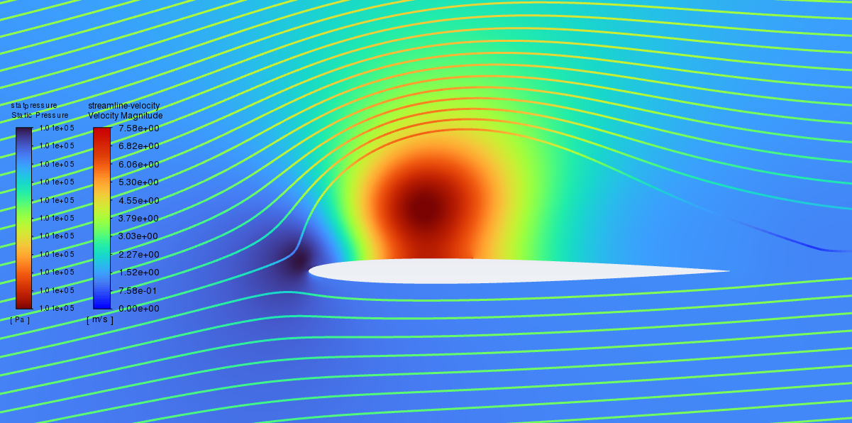
Figure 10&11: Velocity (L) & Pressure (R) Contours - NACA 0006 - AoA 8

Figures 10 & 11 look atypical because the RANS simulation isn’t able to reach a steady state solution because of stall. This is actually quite a close prediction of stall, which can be viewed in the aerodynamic force analysis section of this report.

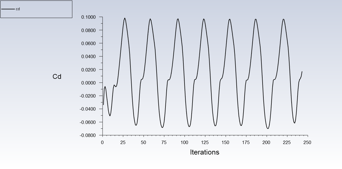
Figure 12&13: Illustration of wild oscillations in the lift (and drag) coefficient at high AoAs due to stall

           Analysis: Aerodynamic Forces

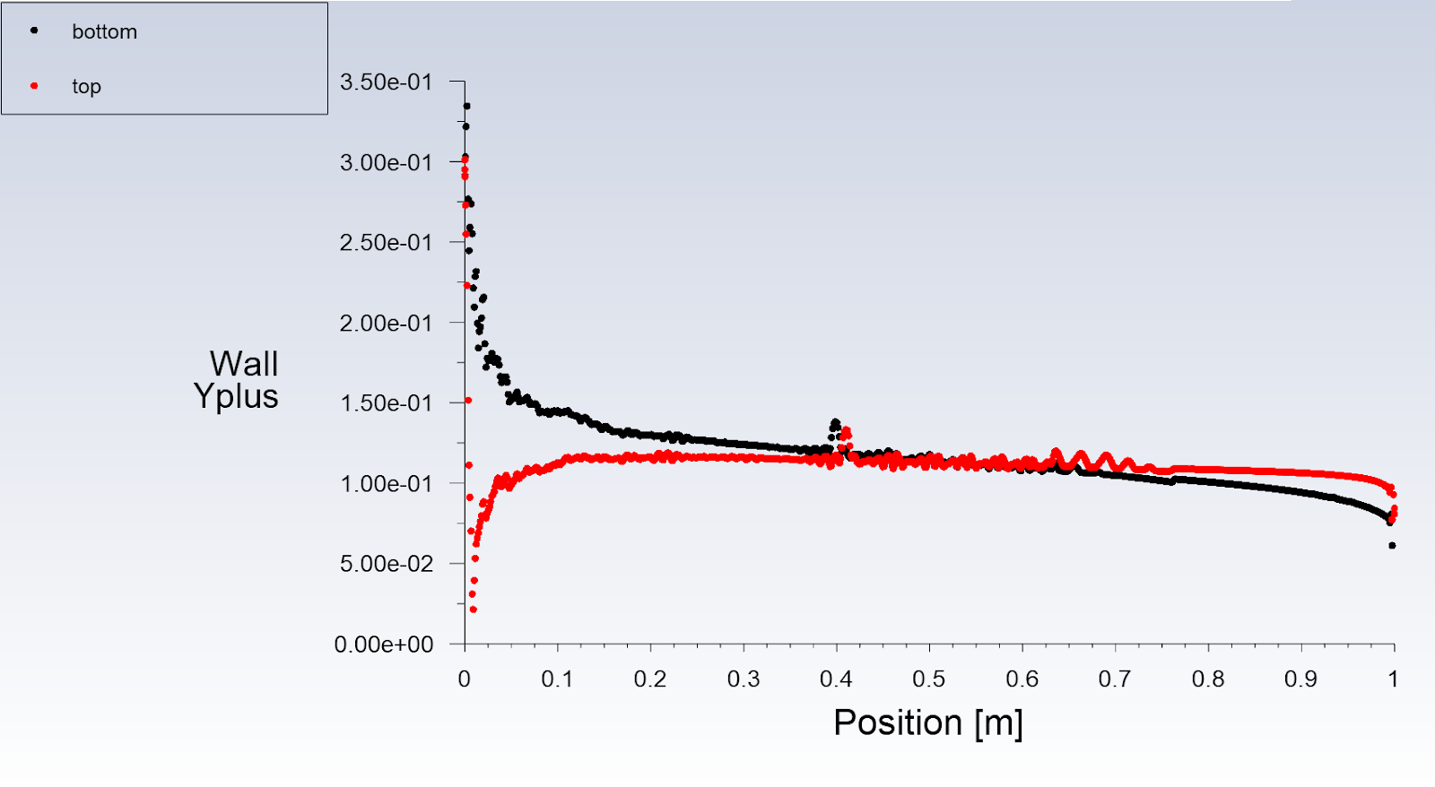
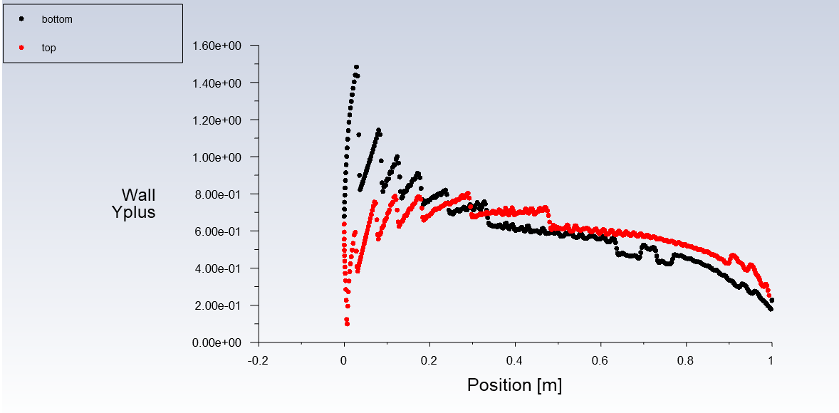
In figures 14-15, we see that as the resolution goes from low to high, the y+ value gets smaller and smaller. For turbulence modeling, y+ on the walls has to be below 1 to get accurate results. Some points on the NACA 2421 have y+ values slightly above 1, as seen in figure 10, but I don’t believe this to be a large enough issue to warrant a rerun of the entire set of simulations.

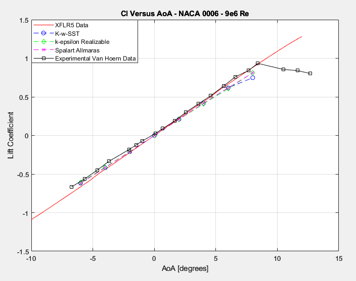
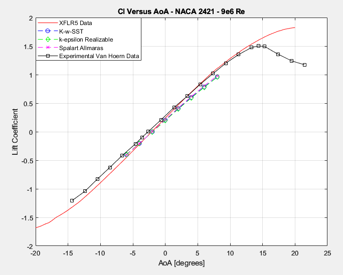
According to figures 16 & 17, the lift predictions from both XFLR5 & RANS CFD seem to correspond pretty well with experimental results. It should be noted that RANS CFD is not particularly well tuned to analyze the unsteady flow patterns near or after stall, so the angle of attack was limited to before stall, however, we can draw the conclusion that despite its accuracy in predicting lift in moderate angles of attack, xfoil’s methodology seems to completely miss the stall point and massively over predicts lift values at higher angles of attack.

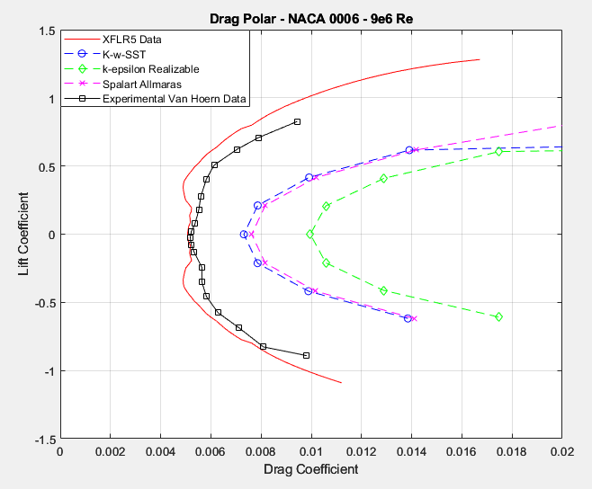
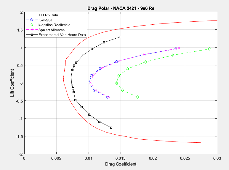
Moving on to drag predictions, the drag polars in figures 18 & 19, illustrate a massive spread. Disappointingly, despite its much higher cost, RANS methods seem to massively over predict drag. Unsurprisingly, the K-w-sst model seems to be the best RANS performer, being closely followed by Spalart Allmaras. However, the author didn’t expect the large difference between the two aforementioned models and k-epsilon. It is somewhat amazing how close the Xfoil viscid/inviscid methodology got in terms of predicted drag values. I would imagine that this trend only holds for incompressible and subsonic flows and that RANS becomes much more accurate when mach numbers are above perhaps 0.3. It is also interesting to note that Xfoil seems to consistently underpredict drag on airfoils, which should be kept in mind during airfoil selection.