Usefulness of Taper Ratio in low to medium Reynolds Number Environments - CFD Analysis

Daniel Samandi

May 16, 2023 • 5 min read

Overview and Objectives

The objective of this study is to determine whether it is efficacious to taper a low-reynolds wing for the purposes of drag reduction. Ordinarily, increasing taper increases the Oswald efficiency of the wing and thereby reduces the induced drag, however, at lower reynolds numbers, tapering a wing leads to critically low reynolds numbers towards the tip of the wing, which tends to reduce the L/D of these wing sections and thereby counteracts the benefits of less induced drag. As previously seen, augmenting standard turbulence models with flow transition predictors produces much higher drag prediction accuracy, which is why the gamma algebraic model was attached to the k-⍵-SST turbulence model in this instance.

Reynolds Number: 300,000
Models: k-⍵-SST with gamma algebraic transition
Steady state solution: final time step
Static pressure: P∞=101325 Pa = 1 atm
Static temperature: T = 300 K
Incompressible: Mach = 0.05
Wing Airfoil: NACA 2412
Primary Wing Dimensions: Characteristic Length = 2 m, Characteristic Area = 20 m^2, AR = 10
Taper Ratio Cases = 1, 0.8, 0.6, 0.4, 0.3

The variations in the wing Geometry can be seen in the list below:

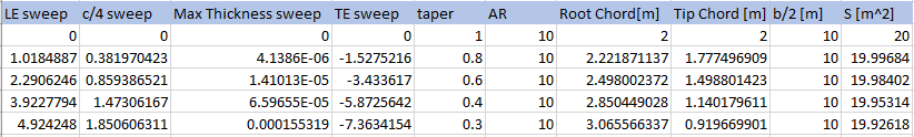
Table 2: Geometric Parameters for Wings

It should be noted that the max thickness sweep (being 40% of the chord for this particular airfoil) was kept as close to zero as possible across the different taper cases in order to eliminate the possible effects of wing sweep.

Furthermore, for all cases the characteristic length and area were kept constant despite small differences evident in table 2.

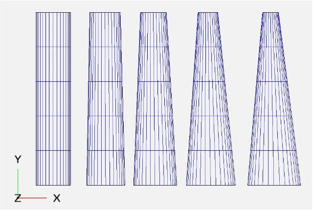
A geometric illustration is also provided below:

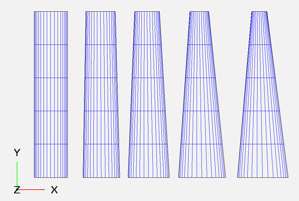
Figure 1: Planform View of Wing Models

Mesh Details

In order to simplify the meshing process and avoid spending days on meshing each of the unique geometries, a simplified meshing approach was utilized, which despite its inefficient use of cells was able to accurately characterize all the flow features, including the boundary layer and freestream.

Number of Cells
Low Resolution	2,415,564
High Resolution	Not Conducted As of Now

Table 2: Number of Cells for each Airfoil Case

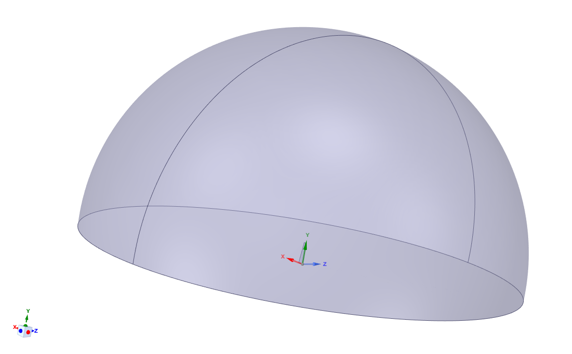
**Figure 2:** Geometry of enclosure and boundary conditions

A half sphere enclosure was used in order to allow changing the angle of attack at the inlet by changing the velocity components in the x and z directions rather than geometrically realigning the wing with respect to the normal freestream flow.

The size of the enclosure is at least 10 span lengths away from the wing in any direction, which should be more than enough for an accurate characterization of freestream conditions similar to an actual flight. The bottom wall was modeled as a zero shear stress wall. The two halves of the sphere are a velocity inlet and a pressure outlet respectively.

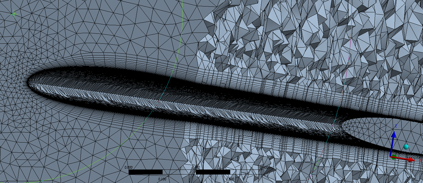
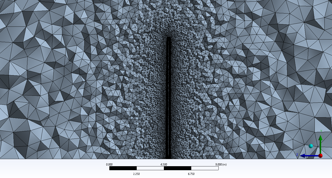
**Figure 3:** 3D view of mesh and boundary layers - Low Resolution

**Figure 4:** Frontal View of Wing Mesh - Low Resolution

It is evident in figures 3-4 that the mesh refinement around the wing in the low resolution run isn’t ideal and has some room for improvement. The high resolution run will be able to confirm spatial convergence of the simulation, however, this has currently not been conducted due to the computational resource scarcity. Other projects currently require more resources, so mesh convergence will have to wait for this project.

**Figure 5:** Surface Pressure y/b = 0.5, λ = 0.3, -2° AoA

**Figure 6:** Surface Pressure y/b = 0.5, λ = 0.3, 6° AoA

Analysis: Aerodynamic Forces

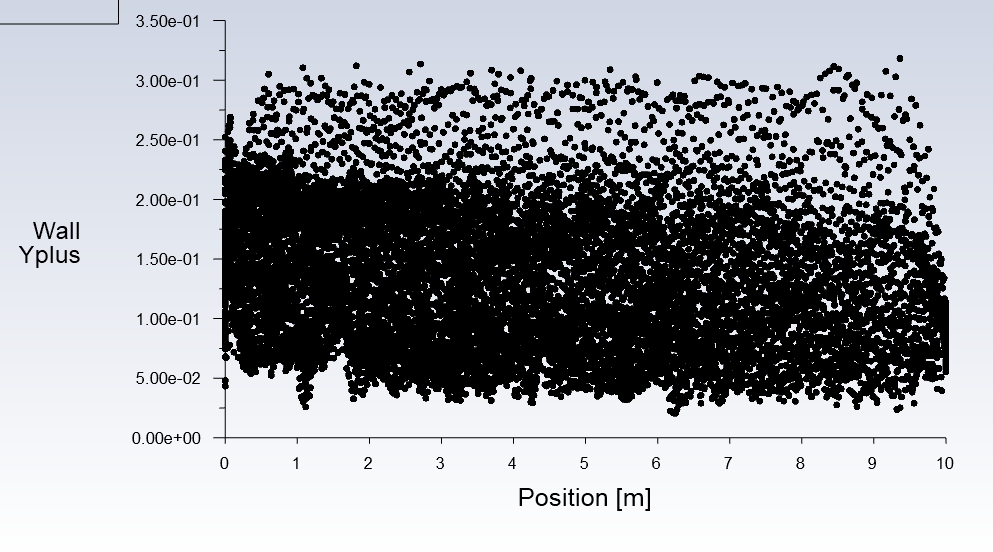
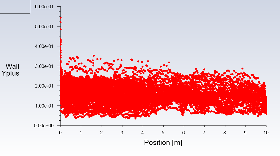
**Figure 7:** Wall y+ vs Span Location, λ = 0.3 , -2° AoA

**Figure 8:** Wall y+ vs Span Location, λ = 0.3 , 6° AoA‌ ‌

According to figures 7-8, it is evident that the boundary layer has been well meshed given that the y+ values are below 1, so we can be sure that the boundary layer has been well resolved and that the skin friction drag component and separation effects are being predicted as accurately as possible given the specific turbulence model

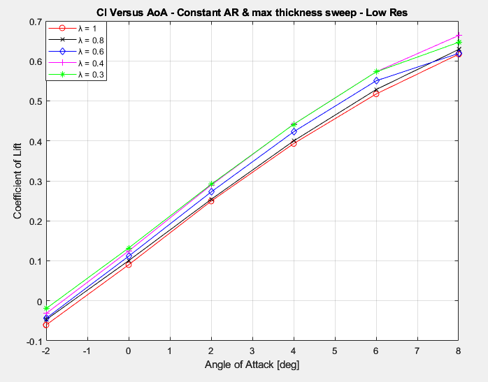
**Figure 9:** Lift Coefficient vs Angle of Attack

It is really interesting to see that there seems to be a consistent offset in terms of the lift produced at a certain angle of attack depending on the taper ratio. This effect is most likely due to the adjustment of the sweep angle in order to keep the max thickness sweep angle at zero across the different wings for compatibility of results (which could have also been done for the quarter chord sweep angle), however, I am not totally sure why this occurs. Given that this effect is consistent across the different angles of attack and taper ratios, I doubt that it is an error with the CFD simulation but is rather probably a physical effect that is avoiding me at the moment.

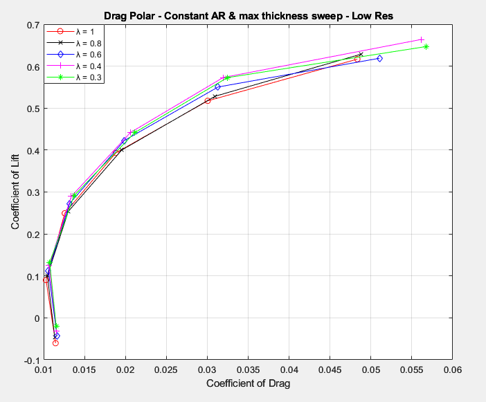
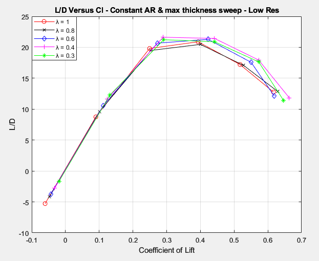
Figures 10 & 11, clearly demonstrate that even at lower Reynolds numbers where a lot of UAVs operate, there seems to be a decent drag reduction by adjusting the lift distribution on the wings through the adjustment of taper ratio. Specifically, according to figure 11, there seems to be a 5-10% increase in L/D between the lowest and highest taper ratios. It should be noted that this L/D increase is probably highly sensitive to the specific airfoil being used as certain airfoils are much more sensitive to Reynolds number changes than others. It could be the case that the NACA 2412 is simply one of the better responding airfoils in this regard.

Sign up for more like this.